Diffusion Models

Origin

Diffusion: image generation based on probability and optimization

Usually we would comprehend diffusion as learning the denoising process of a gaussian distributed noisy image. Alternatively, this video provide a perspective from probability distribution, probing more into how it is “invented”.

Notice: in this part we only talk about diffusion image models that generate good “reasonable” images. We do not let models generate images based on our prompt

probability primer

Probability distribution reflects the likelihood of observing a particular value from a set of values. It can be seen as a function that maps samples to their probability values.

This can be discrete like dice rolling, or continuous like Maxwell distribution. (Specifically, for continuous probability distribution, we refer to the probability function as the density function, and we only define probability based on an infinite subset of the sample space as taking an integral of the density function over this subset)

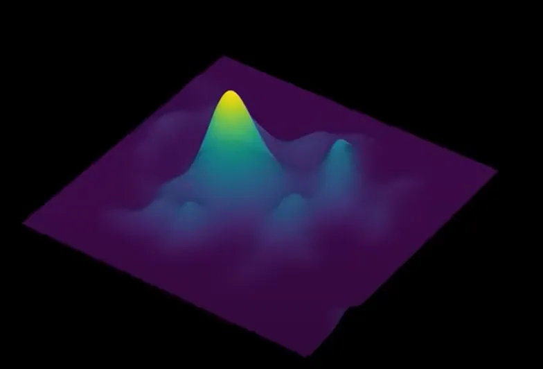
Essentially, image generation can be seen as sampling in the image space, where good images are peaks in the distribution plot

Sampling method

The next problem is: how to sample for an arbitrary distribution? The basis is that we know how to sample from a normal distribution $N(0,1)$ (already implemented in pytorch, ramdom etc.)

The method we use is called Langevein Sampling, which is demonstrated below

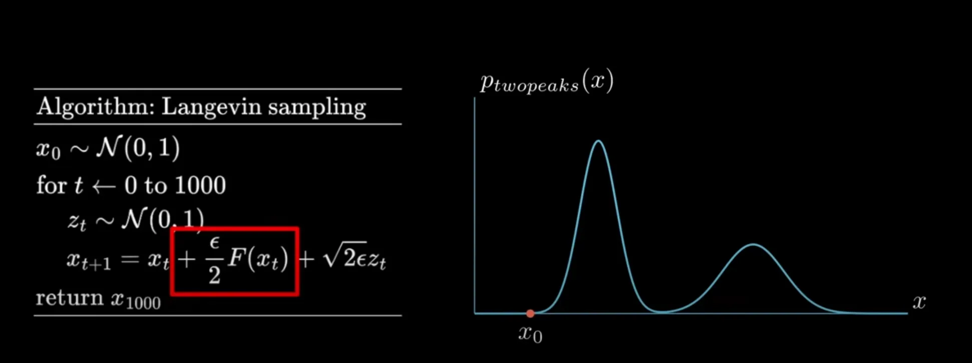There are two components in this sampling method:

1. the gradient function $F$: tells the direction and step that maximizes the probability, which is often set as $\nabla_x (ln (F))$ Calculus knowledge will tell us that $\nabla_x(ln(F))=\frac{\nabla_x F(x)}{F(x)}$, so when $F(x)$ and $\nabla_x F(x)$ are both small, the denominator augments the step that drives the sampling point to “peaks” In the scope of image generation, this factor teaches models to generate “good” images
2. Noize term $z_t$: prevents the sampling method from turning into an “optimization” problem, forcing it to explore the overall landscape and thus sample from other peaks. For image generation, this guarantees diversity in the process. Specifically, image generation is not “optimization”, and diversity is required. For example, we not only want to generate yellow cat images, but also other reasonable cat images like Ragdolls

It can be mathematically proven that the probability distribution of this Langevin sampling will converge to the original probability distribution after sufficiently many times of iteration

[!caution] Coping with the boundaries of the sample space In order to prevent sampling from surpassing the boundaries, we should manually set the gradient function $F$ outside boundaries. Specifically, we would use linear functions for variables outside the boundaries.

Langevin approach to image generation

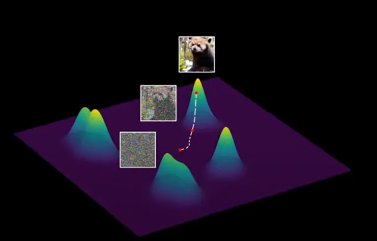
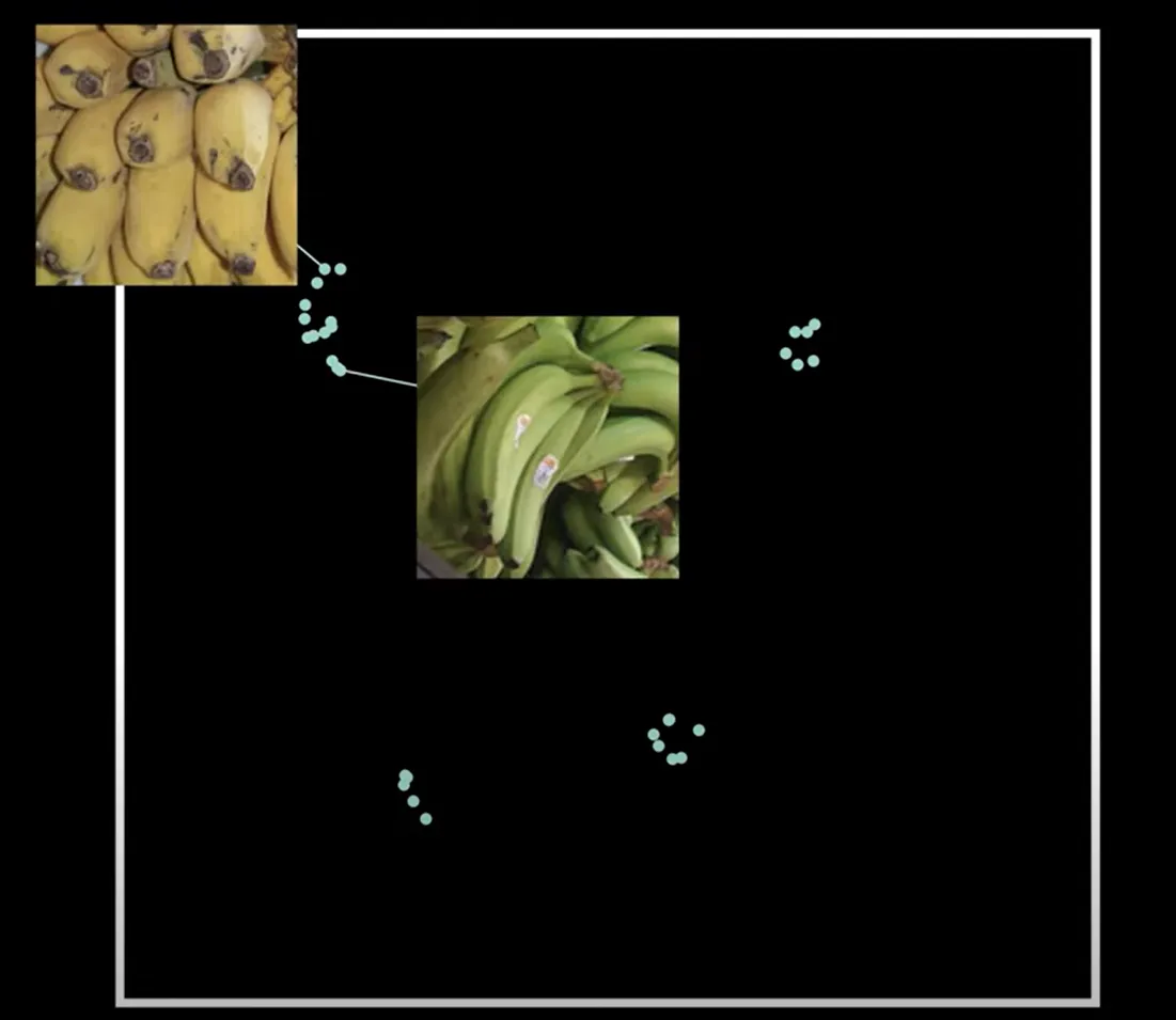
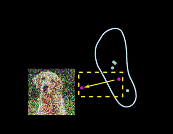
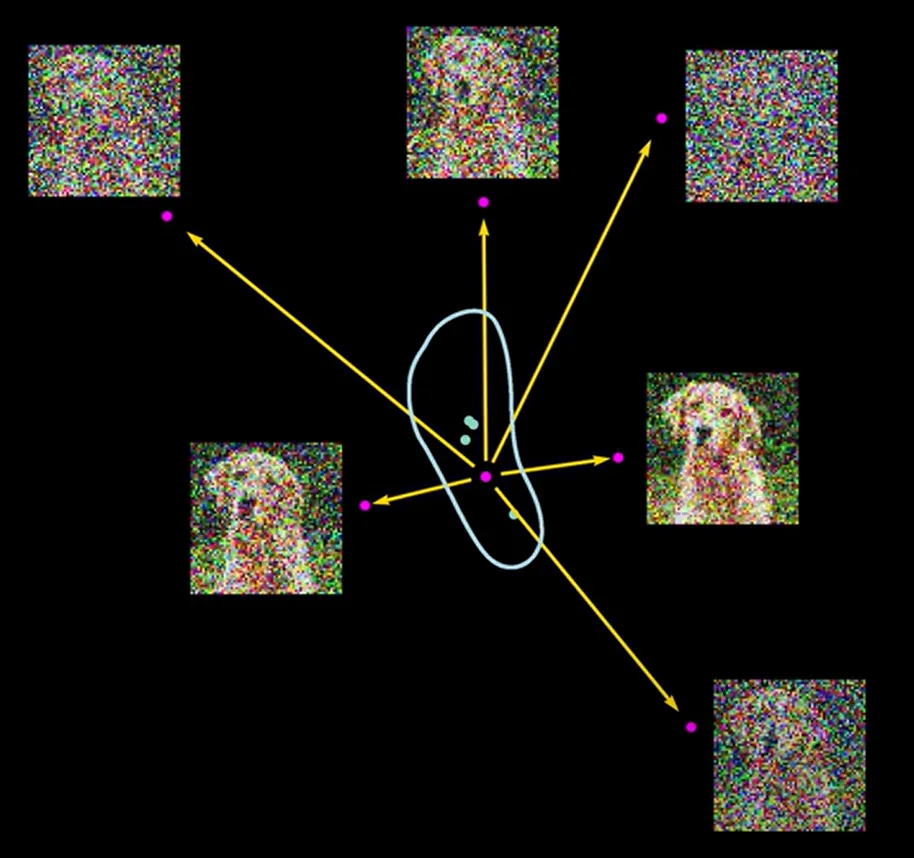
Image space can be seen as a high-dimensional space, where good images tend to concentrate in clusters. However, good images are distributed sparsely as dots in the image space, like what rational numbers are in real numbers 2-D demonstration below:

Diffusion can be viewed as navigating the image space to “good image clusters”

1. Start from a random point in the image space, which will be a pure Gaussian noise
2. Get direction： Models predict a direction towards the “good image cluster”. Notice that the model only points to the local cluster
3. Take a small step in that direction, and take another sample, predict the direction again
4. Iterate this process multiple times, where image gets clearer and clearer

Training and Learning

The training process can be described as “noising” a good image

Get a good image, take a random step to add a bit noise, and you get a supervised pair of “picture-noised picture”, and repeat this multiple times

[!tip] One detail to be mentioned is that the model generates supervised learning pairs automatically, so we only need to feed model the set of good images.

Training details will be added later.

One closer look at the “noising” process

Why do we want to add noise to the denoising process?

A test suggests that removing the noise in Langevin sampling for later steps causes the image to be blurry 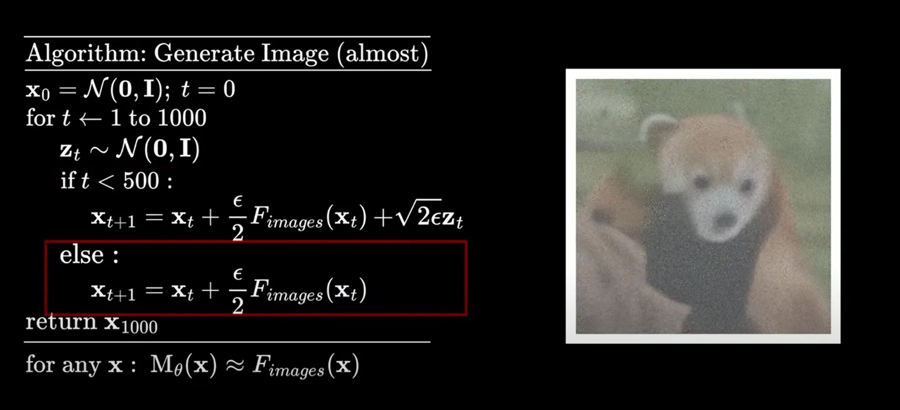This is because the distribution near the good image clusters tend to be very bumpy, with many local minima. Without further noise, sampling will tend to aggregate in the local minimum, getting a blurry image.

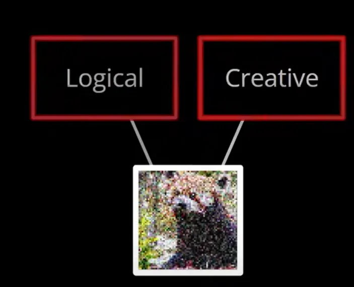
[!tip] Analogy of the role of noise View the gradient and the noise as “logic” and “creative” drawers respectively. “Logic” drawer outlines the logical components of an animal image, while “creative” drawer tends to destroy the drawer’s outlines, allowing the model to focus more on the logic of details. These two work alternatively to get the whole image.