ViT

Learning Vision Transformers—— a pure transformer CV model

Summary of Previous Works

Previously, transformer has been quite successful and widely applied on NLP tasks, featuring its dramatic improvement after scaling up.

However, CNN is still dominant on CV tasks. Attempts to apply transformers into CV tasks can be divided into two categories:

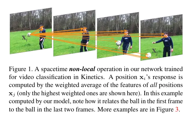
1. Enhancing CNNs with Transformers: like Non-local NNs (non-local modules that calculate “attention” between distant pixels) and Detection Transformers (CNN+ Transformers)
2. Pure Attention models: the Stand-Alone Self-Attention Vision Models published in 2019 completely substitutes self-attention layers for convolutional layers. It has achieved a rivalling performance to traditional CNNs. Further, Axial-DeepLab proposes axial attention that respectively performs 1D attention on multiple axises.

Critique of Previous work

Previous models have low computational efficiency, and are not compatible with scaling up Traditional CNN layers has a very low computational efficiency (experiment in this paper suggests that ViT are 4x more efficient than CNNs) Pure Self-Attention Models own a complexity of $N^2$ (Where N is the number of pixels in a picture), so it is too heavy for scaling up Unlike transformer models that utilizes accelerated kernels for matrix multiplication, Models like Non-local Models and Axial Attention requires specific acceleration algorithms that are difficult to implement on GPUs, and therefore computes very slowly on GPUs.

What the dissertation does

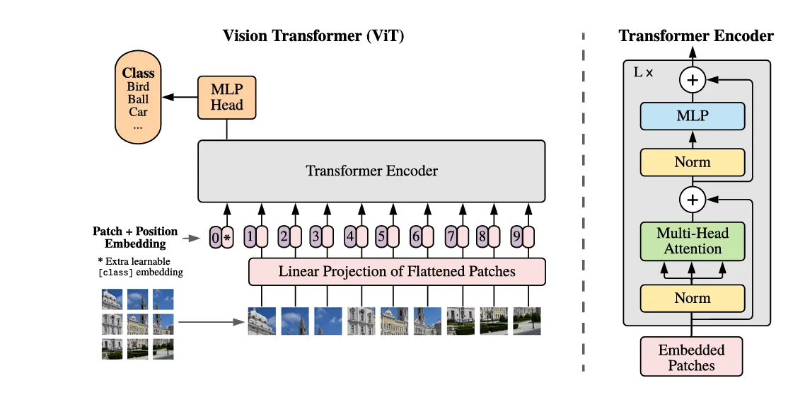
In this paper, the researcher proposes a vision Transformer model that can scale up based on current transformer kernels on GPUs. This ViT does little modification on the NLP transformers, and preserves the Transformer encoder.

Further, this work explores image recognition at larger scales than the standard ImageNet, focusing on ImageNer-21k and JFT-300M as datasets

Method

Actually, compared to NLP transformers, Vision transformers only modify the input sequence for pictures

Mathematically, one image have a resolution of $H\times W$ and $C$ channels (for RGB that’s 3), and we have one image as the 3D input $x\in \mathbb{R}^{H\times W\times C}$

Step 1: Image Patching and Flattening

Reshape x into a sequence of 2-D photo patches, and each photo patch is resized into a 1-D vector Assume that the patch size is D, then the result is $x_{p}\in \mathbb{R}^{N\times (C \cdot P^2)}\ (N=H*W/P^2)$

Step 2: Linear projection

Modern transformer often project vector inputs of dimension $L$ into lower-dimension $D$ before feeding them into attention blocks, so we have a projection matrix $E_{p}\in \mathbb{R}^{CP^2\times D}$ , and the results will be $x_p\times E_p=x_d\in \mathbb{R}^{N\times D}$

Step 3: [class] embedding and positional embedding

3.1: [class] embedding This process adds a learnable embedding vector $x_{class}$ to the beginning of the input sequence $x_d$ that serves as the final representation of the whole sequence input When the sequence passes through the Transformer encoder, the added vector $x_{class}$ interacts and absorbs attention from all image patch tokens, and after encoding layers, it becomes the vector $z_0^L$ sent to the prediction process

After this process the input tensor x becomes $x_d'\in \mathbb{R}^{(N+1)\times D}$

3.2 Positional Embedding

This means adding a matrix $E_{pos}\in \mathbb{R}^{(N+1)\times D}$ that preserves the order and spatial information of each vector in the sequence. This can be interpreted as a unique and learnable vector for every position in the input sequence.

Without this positional embedding, the model will not pay attention to the order and spatial information of the input sequence. Further, this paper points out that transformers lack understanding and awareness of locality as CNNs do , so this positional embedding is crucial to retain spatial information

outcome is $z^0=x_d' + E_{pos}$ as the input for encoder

Step 4: Transformer encoder: MSAs + MLPs

Consists of multiple MSA( multi-head self-attention layer) and MLPs coupled with Layer-norms Specifically, ResNet connection is applied after every MSA and MLP, so the outcome will be $z^1=z^0+MSA(z^0);z^2=z^1+MLP(z^1)$

After passing multiple blocks, the final output is $z^L$, and the vector at position 0 (originally the added class vector) is selected as the representation of the input for further prediction

Step 5: Classification Head

5.0:Normalization Apply a LayerNorm to $z_0^L$

5.1: Pre-training stage The ViT model is first pretrained on a large dataset JFT-300M. The pre-trained model is a 2-layer MLP, whose outcome is the number of class in JFT-300M (possibly 18000)

5.2: Fine-tuning stage

When applying models to smaller datasets like ImageNet or CiFaR-10, the original classification head is replaced by a new classification head as a single feed-forward Layer that is initialized as all-zero

This Linear layer has a weight matrix $E_{pred}\in \mathbb{R}^{D\times K}$, with a final output logit $y\in R^{1\times K}$ that is translated into probability distribution through softmax

Methods summary

Actually the only modification of ViT on NLP transformers is converting the image into a sequence of photo patches. The transformer encoders, especially self-attention layers remain unchanged, so the previous acceleration methods on GPUs are still applicable for this model. Thus it is much easier to scale up than many other models

Experiments